BEELINE
Overview
BEELINE provides a set of tools for evaluating methods that infer gene regulatory networks (GRN) from single-cell gene expression data. The BEELINE framework is divided into the following modules:
- BLRun package : contains the BEELINE’s Runner module, a Python wrapper for 12 GRN inference algorithms with options to add new methods.
- BLEval package : contains the BEELINE’s Evaluation module that provides easy-to-use tools for evaluating GRN reconstructions.
- BLPlot package : contains the BEELINE’s plotting module for visualizing output from BLEval.
Getting Started
The BEELINE pipeline interfaces with the implementations of various
algorithms through Docker containers. BEELINE natively supports Debian-based distributions (e.g. Ubuntu), and also supports Windows/other Linux distributions. Install Docker Engine for your system.
If you prefer/your system supports a graphical interface, you may instead install Docker Desktop.
Tip
Setup docker to run docker without using sudo each time by adding yourself to the Docker group. You may have to restart your shell for the changes to take effect.
sudo usermod -aG docker $USER
See more details here.
Once docker has been set up correctly, the next step is to create the docker containers for each of the algorithms. The script initialize.sh builds these containers. Run the following in the terminal
. initialize.sh
Note
This step will take a while! Ensure that your system also has ~20GB of memory available to build each image.
BEELINE requires Miniconda (or Anaconda) for package management. Run the following command to automatically create an Anaconda virtual environment named BEELINE that contains all the necessary dependencies.
. setupAnacondaVENV.sh
Tip
Anaconda isolates different sets of dependencies into each environment that it creates. To use an environment, you must "activate" it. You may have to reactivate it after logging back into a server or switching to another environment with
conda activate BEELINEBEELINE should now be installed and ready to run benchmarks.
To compute proposed reconstructions using the 12 GRN algorithms on the example dataset, run
python BLRunner.py --config config-files/config.yaml
To compute areas under the ROC and PR curves for the proposed reconstructions, run
python BLEvaluator.py --config config-files/config.yaml --auc
To display the complete list of evaluation options, run
python BLEvaluator.py --help
Tutorial
This tutorial will first explain the structure of the BEELINE repository, with a walkthrough of the different components that the user can customize.
Project outline
The BEELINE repository is structured as follows:
BEELINE
|-- inputs/
|   `-- examples/
|       `-- GSD/
|           |--refNetwork.csv
|           |--PseudoTime.csv
|           `--ExpressionData.csv
|-- config-files/
|   `-- config.yaml
|-- BLRun/
|   |-- sinceritiesRunner.py
|   `-- ...
|-- BLPlot/
|   |-- NetworkMotifs.py
|   `-- CuratedOverview.py
|-- BLEval/
|   |-- parseTime.py
|    `-- ...
|-- Algorithms/
|     |-- SINCERITIES/
|     `-- ...
|-- LICENSE
|-- initialize.sh
|-- BLRunner.py
|-- BLEvaluator.py
|-- README.md
`-- requirements.txt
Input Datasets
The sample input data set provided is generated by BoolODE using the Boolean model of Gonadal Sex Determination as input. Note that this dataset has been pre-processed to produce three files that are required in the BEELINE pipline.
- ExpressionData.csv contains the RNAseq data, with genes as rows and cell IDs as columns. This file is a required input to the pipline. Here is a sample ExpressionData.csv file
- PseudoTime.csv contains the pseudotime values for the cells in ExpressionData.csv. We recommend using the Slingshot method to obtain the pseudotime for a dataset. Many algorithms in the pipeline require a pseudotime file as input. Here is a sample PseudoTime file.
- refNetwork.csv contains the ground truth network underlying the interactions between genes in ExpressionData.csv. Typically this network is not available, and will have to be curated from various Transcription Factor databases. While this file is not a requirement to run the base pipeline, a reference network is required to run some of the performance evaluations in BLEval package. Here is a sample refNetwork.csv file
The figure below shows the t-SNE visualization of the expression data from the example dataset.
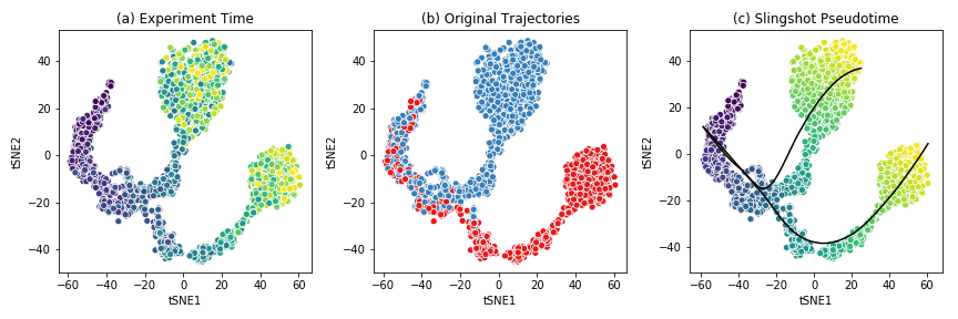
This dataset shows a bifurcating trajectory, as is evidenced by the part (a) of the figure, where each ‘cell’ is colored by the timepoint at which it was sampled in the simulation (the darker colors indicate earlier time points). Clustering the simulation confirms the two trajectories, indicated in red and blue respectively in part (b). Finally, running Slingshot on this dataset and specifying the cluster of cells corresponding to the early time points yields two pseudotime trajectories, shown in part (c). For details on the generation of this simulated dataset, see BoolODE.
Attention
Please ensure that any input dataset you create is comma separated, and contains the correct style of column names.
Config files
Beeline uses YAML files to allow users to flexibly specify inputs and algorithm run parameters. A sample config file is provided in here. A config file should contain at minimum
input_settings:
    input_dir : "Base input directory name, relative to current working directory (recommended: inputs)"
    dataset_dir: "Subdirectory of input_dir where the datasets are placed in"
    datasets:
        - name: "Dataset name"
          exprData: "Expression Data filename"
          cellData: "PseudoTime filename"
          trueEdges: "Ground truth network filename"
    algorithms:
        - name: "Algorithm name"
          params:
              # Any other parameters that can be passed to
              # this algorithm
              should_run: [True] # or False

output_settings:
    output_dir : "Base output directory name, relative to current working directory (recommended: outputs)"
    output_prefix: "Prefix for writing evaluation summary files"
Apart from indicating the path to the base directory and the specific folder containing the input, the config file indicates which algorithms should be run, along with the parameters to be passed to the algorithms, if any. For a list of parameters that the pipeline currently passes to the algorithms, see Details of supported algorithms. Finally, the YAML file also specifies the output_dir where the outputs are written. Note that the output directory structure under output_dir is same as the input directory strucutre under input_dir. For example, if the config file contains the following:
input_settings:
    input_dir : "inputs"
    dataset_dir: "example"
    datasets:
        - name: "GSD"
          exprData: "ExpressionData.csv"
          cellData: "PseudoTime.csv"
          trueEdges: "refNetwork.csv"
    algorithms:
        - name: "PIDC"
          params:
              should_run: [True]
        - name: "SCODE"
          params:
              should_run: [False]
              z: [10]
              nIter: [1000]
              nRep: [6]

output_settings:
    output_dir : "outputs"
    output_prefix: "GSD"
BEELINE would interepret this as follows:
- The input expression data file is located at
inputs/example/GSD/ExpressionData.csv, the pseudotime file is located atinputs/example/GSD/PseudoTime.csv, and the reference network or true edges file is located atinputs/example/GSD/refNetwork.csv. Note that the paths are relative to the current working directory. - The algorithm specific inputs will be placed under
inputs/example/GSD/<algorithm_name>. For example, for PIDC, the inputs will be placed underinputs/example/GSD/PIDC/. The SCODE algorithm will be skipped becuase the should_run flag is set to False. - The output folder structure will be similar to that of the inputs under output_dir. For example, the outputs obtained after running PIDC on this dataset will be placed under
outputs/example/GSD/PIDC/.
Attention
Please ensure that the YAML file is correctly indented!
Running the pipeline
Once the input dataset has been generated and formatted as described
in Section Input Datasets , and the config file has been
created as described in Config files, the pipeline can be
executed by simply calling BLRun.py with the config file
specifying the inputs and the algorithms to run, passed using the
--config option which takes the path to the config file.
To run the pipeline, simply invoke
python BLRunner.py --config PATH/TO/CONFIG/FILE
For details about the implementation of BLRun , see blrunguide .
Running the evaluation scripts
Each algorithm outputs an inferred network in the form of a ranked edge list. BEELINE implements a consistent interface using the config file in order to retrieve the predictions of multiple algorithms and evaluate them using a variety of methods.
The evaluation of the inferred networks is done by calling the
BLEvaluator.py script. Like the BLRunner.py script, the
Evaluator script takes the config file as input. Every subsequent
option passed to this script calls a different evaluation script. For instance,
in order to analyze the AUROC and AUPRC values, and also analyze network motifs,
use the following command
python BLEvaluator.py --config PATH/TO/CONFIG/FILE \
                           --auc \ # calls the computeAUC script
                           --motifs \ # calls the computeNetMotifs script
The full list of available evaluation functions and their corresponding options to
be passed to BLEvaluator.py are given below:
| -h, –help | show the help message and exit |
| -c, –config <file-name> | Configuration file containing list of datasets, algorithms, and output specifications. |
| -a, –auc | Compute median of areas under Precision-Recall and ROC curves. Calls BLEval.computeAUC. |
| -j, –jaccard | Compute median Jaccard index of predicted top-k networks
for each algorithm for a given set of datasets generated from the same
ground truth network. Calls BLEval.computeJaccard. |
| -r, –spearman | Compute median Spearman Corr. of predicted edges for each algorithm for a given set of datasets generated from the same ground truth network. Calls BLEval.computeSpearman. |
| -t, –time | Analyze time taken by each algorithm for a. Calls BLEval.parseTime. |
| -e, –epr | Compute median early precision. Calls BLEval.computeEarlyPrec. |
| -s, –sepr | Analyze median (signed) early precision for activation and inhibitory edges. BLEval.computeSignedEPrec. |
| -m, –motifs | Compute network motifs in the predicted top-k networks. Calls BLEval.computeNetMotifs |
For details about the implementation of BLEval , see Adding a new evaluation technique .
Details of supported algorithms
The following table lists the algorithms and the parameters they take as input, along with the default parameter values
| Algorithms | Input Parameters |
|---|---|
| SINCERITIES |
|
| SCODE |
|
| SCNS | None |
| SCINGE |
|
| PPCOR |
|
| PIDC | None |
| LEAP |
|
| SCRIBE |
|
| GRNVBEM | None |
| GRISLI |
|
| GENIE3 | None |
| GRNBOOST2 | None |
Developer Guide
Please follow the following steps to add a new GRN inferenmence method to BEELINE.
Adding a new GRN inference method
In order to ensure easy set-up and portability, all the GRN algorithms in BEELINE are provided within their own separate Docker instances. This also avoids conflicting libraries/software versions that may arise from the GRN algorithm implmentations. More resources on Docker can be found here. In order to add a new GRN method to BEELINE, you will need the following components.
- Create a Dockerfile: To create a Docker image for your GRN algorithm locally, you will need to start with a “Dockerfile” that contains necessary software specifications and commands listed in a specific order from top to bottom. BEELINE currently provides Dockerfiles for GRN implementations in Python, R, MATLAB, and Julia. These Dockerfiles can be used as a template for adding other GRN algorithms. Note that in order to run MATLAB-based code, we recommend first builing a standalone MATLAB application for your GRN algorithm MATLAB Runtime and then setting up your Dockerfile to simply execute the pre-compiled binaries. For example, the Dockerfile using R which runs the script runPPCOR.R within the Docker container is as follows:
FROM r-base:3.5.3 #This is the base image upon which necessary libraries are installed

LABEL maintainer = "Aditya Pratapa <adyprat@vt.edu>" #Additional information

RUN apt-get update && apt-get install time #Installl time command to compute time taken

USER root #Set main user as root to avoid permission issues

WORKDIR / #Sets current working directory

RUN R -e "install.packages('https://cran.r-project.org/src/contrib/ppcor_1.1.tar.gz', type = 'source')" #Installs a specific version of PPCOR package

COPY runPPCOR.R / #Copy the main R script which will perform necessary GRN computations

RUN mkdir data/ #Make a directory to mount the folder containing input files
The Dockerfile must then be placed under the Algorithms/<algorithm-name> folder in BEELINE. Then the following lines must be added to the initialize.sh script.
cd $BASEDIR/Algorithms/<algorithm-name>/
docker build -q -t <algorithm-name>:base .
echo "Docker container for <algorithm-name> is built and tagged as <algorithm-name>:base"
Replace <algorithm-name> with the name of the new algorithm that is being added to BEELINE.
2. Create a <algorithm-name>Runner.py script: Once the Docker image is built locally using the above Dockerfile, we will then need to setup a BLRun object which will read necessary inputs, runs GRN algorithm inside the Docker image, and finally parses output so that evaluation can be performed using BLEval.
Most of the GRN algorithms in BEELINE require a gene-by-cell matrix provided as input, along with a pesudotime ordering of cells, and any additional manually specified parameters. These details are specified as inputs to BEELINE using Config files as mentioned earlier. In our current implementation, we provide a separate csv file for expression matrix and pseudotime files, whereas algorithm parameters are specified as command line arguments. However, this can be modified easily to specify even the parameters using a separate file by simply providing its path in the config file. Each <algorithm-name>Runner.py script should contain the following three functions:
generateInputs(): This function reads the two input data files (i.e., expression data and the pseudotime), and processes them into the format required by the given algorithm. For example, the algorithm may only require the cells in the expression matrix to be ordered in pseudotime, instead of exact pesudotime values as input. Moreover, if the algorithm requires that you run the GRN inference on each trajectory separately, we can this function to write the separate expression matrices contianing only cells of a particular trajectory.run(): This function constructs a “docker run” system command with the appropriate command line parameters to be passed to the docker container in order to run a given algorithm. The docker run command also needs to mount the folder containing the input files using the “-v” flag and specify where the outputs are written. If the algorithm needs to be run separately on each trajectory, it can be simply called in a loop inside this function.parseOutput(): This function reads the algorithm-specific outputs and formats it into a ranked edgelist comma-separated file in the following format which can be subsequently used byBLEval
Gene1,Gene2,EdgeWeight
reg1,targ1,edgeweight
where the first line are the column names, and the subsequent lines contain the edges predicted by the network. The Gene1 column should contain regulators, the Gene2 column the targets, and EdgeWeight column the absolute value of the weight predicted for edge (regulator,target). Note that in cases where the algorithm requires that you run the GRN inference on each trajectory separately, a single output network is obtained by finding the maximum score for a given edge across the GRNs computed for each individual trajectory. Please ensure that all of the above three functions in your script accept arguments of type BLRun.runner.Runner. The <algorithm-name>Runner.py script must then be placed under the BLRun/ folder in BEELINE.
- Add the new alorithm to runner.py: The next step is to integrate the new algorithm within
BLRunobject. This can be achieved by adding the above three modules from the above step, i.e,generateInputs(),run(), andparseOutput()to runner.py. - Add the new alorithm to config.yaml: The final step is to add the new algorithm and any necessary parameters to the cofig.yaml. Note that currently BEELINE can only handle one parameter set at a time eventhough multiple parameters can be passed onto the single parameter object.
algorithms:
    - name: <algorithm-name>
      params:
          # Any parameters that can be passed to this algorithm
          paramX: [0.1]
          paramY: ['Text']
          should_run: [True] # or False
Adding a new evaluation technique
BEELINE currently supports several evaluation techniques, namely, area under ROC and PR curves, eary precision, early signed precision, time and memory consumption, network motifs, jaccard similarities, and spearman coefficients. A new evaluation technique can be easily added to BEELINE using the following procedure.
- Add the script containing the new evaluation technique to the BLEval/ folder.
- The next step is to integrate the new technique into the
BLEvalobject. This can be achieved by adding it as a new module underBLEvalin the BLEval/__init__.py script. Please ensure that your script can accept arguments of typeBLEval. - The final step is to add a command line option to perform the evaluation to BLEvaluator.py.
API Reference
- BLRun package
- Submodules
- BLRun.genie3Runner module
- BLRun.grisliRunner module
- BLRun.grnboost2Runner module
- BLRun.grnvbemRunner module
- BLRun.jump3Runner module
- BLRun.leapRunner module
- BLRun.pidcRunner module
- BLRun.ppcorRunner module
- BLRun.runner module
- BLRun.scingeRunner module
- BLRun.scnsRunner module
- BLRun.scodeRunner module
- BLRun.scribeRunner module
- BLRun.sinceritiesRunner module
- BLEval package
- BLPlot package