Running BEELINE
This section describes how to prepare inputs, configure, and run the BEELINE pipeline end-to-end.
Input Datasets
The sample input data set provided is generated by BoolODE using the Boolean model of Gonadal Sex Determination as input. Note that this dataset has been pre-processed to produce three files that are required in the BEELINE pipeline.
ExpressionData.csv contains the RNAseq data, with genes as rows and cell IDs as columns. This file is a required input to the pipeline. Here is a sample ExpressionData.csv file
PseudoTime.csv contains the pseudotime values for the cells in ExpressionData.csv. We recommend using the Slingshot method to obtain the pseudotime for a dataset. Many algorithms in the pipeline require a pseudotime file as input. Here is a sample PseudoTime file.
GroundTruthNetwork.csv contains the ground truth network underlying the interactions between genes in ExpressionData.csv. Typically this network is not available, and will have to be curated from various Transcription Factor databases. While this file is not a requirement to run the base pipeline, a reference network is required to run some of the performance evaluations in BLEval package. Here is a sample GroundTruthNetwork.csv file
The figure below shows the t-SNE visualization of the expression data from the example dataset.
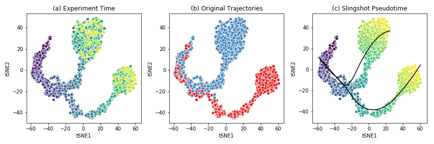
This dataset shows a bifurcating trajectory, as is evidenced by the part (a) of the figure, where each ‘cell’ is colored by the timepoint at which it was sampled in the simulation (the darker colors indicate earlier time points). Clustering the simulation confirms the two trajectories, indicated in red and blue respectively in part (b). Finally, running Slingshot on this dataset and specifying the cluster of cells corresponding to the early time points yields two pseudotime trajectories, shown in part (c). For details on the generation of this simulated dataset, see BoolODE.
Attention
Please ensure that any input dataset you create is comma separated, and contains the correct style of column names.
Config Files
Beeline uses YAML files to allow users to flexibly specify inputs and algorithm run parameters. A sample config file is provided here. A config file should contain at minimum
input_settings:
    input_dir : "Base input directory (recommended: inputs)"
    datasets:
        - dataset_id: "Dataset group label"
          should_run: [True]
          groundTruthNetwork: "Ground truth network filename"
          runs:
              - run_id: "Run subdirectory name"
    algorithms:
        - algorithm_id: "Algorithm name"
          image: "Docker image tag"
          should_run: [True]  # or [False]
          params:
              # Any algorithm-specific parameters

output_settings:
    output_dir : "Base output directory (recommended: outputs)"
Apart from indicating the path to the base input directory, the config file
specifies which datasets and runs to process, which algorithms should be run,
and the parameters to pass to each algorithm. For a list of parameters
that the pipeline currently supports, see Supported Algorithms. The config
also specifies output_dir, where all outputs are written.
The datasets list groups runs that share the same ground truth network
under a common dataset_id. Each run_id corresponds to a
subdirectory of input_dir/dataset_id/ containing the expression,
pseudotime, and ground truth files for that replicate.
For example, if the config file contains:
input_settings:
    input_dir : "inputs"
    datasets:
        - dataset_id: "GSD"
          should_run: [True]
          groundTruthNetwork: "GroundTruthNetwork.csv"
          runs:
              - run_id: "GSD-1"
    algorithms:
        - algorithm_id: "PIDC"
          image: "grnbeeline/pidc:base"
          should_run: [True]
          params: {}
        - algorithm_id: "SCODE"
          image: "grnbeeline/scode:base"
          should_run: [False]
          params:
              z: [10]
              nIter: [1000]
              nRep: [6]

output_settings:
    output_dir : "outputs"
BEELINE would interpret this as follows:
The input files for run
GSD-1are located atinputs/GSD/GSD-1/, e.g.inputs/GSD/GSD-1/ExpressionData.csv. The ground truth network is read frominputs/GSD/GSD-1/GroundTruthNetwork.csv.SCODE will be skipped because
should_runis set to[False].Outputs for each algorithm are written under
outputs/GSD/GSD-1/<algorithm_id>/. For example, PIDC results will be atoutputs/GSD/GSD-1/PIDC/rankedEdges.csv.
Attention
Please ensure that the YAML file is correctly indented!
Running the Pipeline
Once the input dataset has been generated and formatted as described
in Section Input Datasets, and the config file has been
created as described in Config Files, the pipeline can be
executed by calling BLRunner.py with the config file
passed using the --config option.
To run the pipeline, simply invoke
python BLRunner.py --config PATH/TO/CONFIG/FILE
For details about the implementation of BLRun, see Adding a new GRN inference method.
Running the Evaluation Scripts
Each algorithm outputs an inferred network in the form of a ranked edge list. BEELINE implements a consistent interface using the config file in order to retrieve the predictions of multiple algorithms and evaluate them using a variety of methods.
The evaluation of the inferred networks is done by calling the
BLEvaluator.py script. Like BLRunner.py, the
evaluator script takes the config file as input. Every subsequent
option passed to this script calls a different evaluation script. For instance,
in order to analyze the AUROC and AUPRC values and also analyze network motifs,
use the following command
python BLEvaluator.py --config PATH/TO/CONFIG/FILE \
                           --auc \   # calls the computeAUC script
                           --motifs  # calls the computeNetMotifs script
The full list of available evaluation functions and their corresponding options
to be passed to BLEvaluator.py are given below:
-h, –help |
show the help message and exit |
-c, –config <file-name> |
Configuration file containing list of datasets, algorithms, and output specifications. |
-a, –auc |
Compute median of areas under Precision-Recall and ROC curves. Calls |
-j, –jaccard |
Compute median Jaccard index of predicted top-k networks
for each algorithm for a given set of datasets generated from the same
ground truth network. Calls |
-r, –spearman |
Compute median Spearman Corr. of predicted edges for each algorithm for a given set of datasets generated from the same ground truth network. Calls |
-t, –time |
Analyze time taken by each algorithm. Calls |
-e, –epr |
Compute median early precision. Calls |
-s, –sepr |
Analyze median (signed) early precision for activation and inhibitory edges. Calls |
-m, –motifs |
Compute network motifs in the predicted top-k networks. Calls |
-p, –paths |
Compute path length statistics on the predicted top-k networks. Calls |
-b, –borda |
Compute edge ranked list using the various Borda aggregation methods. Calls |
For details about the implementation of BLEval, see Adding a new evaluation technique.
Running the Plotter Script
Once evaluation has been run with BLEvaluator.py, results can be
visualised by calling BLPlotter.py with the same config file and an
output directory for the generated plots.
python BLPlotter.py --config PATH/TO/CONFIG/FILE --output PATH/TO/OUTPUT/DIR
The full list of available plot types and their corresponding options are given below:
-h, –help |
show the help message and exit |
-c, –config <file-name> |
Configuration file containing list of datasets and algorithms. The same file used with BLEvaluator.py may be used here. |
-o, –output <dir> |
Output directory for generated plots (default: current directory). |
-a, –auprc |
Produce per-dataset AUPRC plots ( |
-r, –auroc |
Produce per-dataset AUROC plots ( |
-e, –epr |
Produce a box plot of early precision values for the evaluated algorithms ( |
–summary |
Produce a heatmap of median AUPRC ratios and median Spearman stability per algorithm and dataset ( |
–epr-summary |
Produce a heatmap of median AUPRC ratio, EPR ratio, and signed EPR ratios per algorithm and dataset ( |
–all |
Run all plots. |